Robert E. West

Most of my time as a graduate student at UVA has been spent working on HotSpot 7.0, a pre-RTL thermal simulator. This work has resulted in two published papers, "Extending HotSpot to Model Microfluidic Cooling" in SRC's TECHCON 2020, and "Modeling Microfluidic Cooling in HotSpot" in GOMACTech 2021. Below I talk about how HotSpot 6.0 works and about the new features and functionality that I've added to the next release, HotSpot 7.0.

HotSpot 6.0

HotSpot is a pre-RTL thermal simulator. That means that it doesn't need any information about how a chip actually works; it doesn't care what kind of fast adder circuits are being used or whether the CPU is out-of-order or not. It just needs to know what the parts of the chip are (commonly called the floorplan) and how much power they dissipate. It's common to use a tool like McPAT to get this power information. Once HotSpot knows a chip's floorplan and its power dissipation, it runs a thermal simulation and gives the user the temperatures throughout the chip.

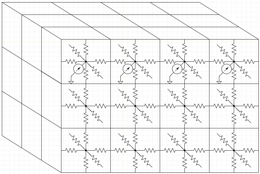
HotSpot works by dividing an entire chip into an array of 3D cells. Then, each cell is modeled as a node in a thermal circuit. A thermal circuit is analogous to an electrical circuit, but the quantities involved are different: temperature is used in place of voltage, heat flow in place of current flow, and thermal resistance in place of electrical resistance. Each cell in the chip is modeled as a different node in this circuit. The ability for heat to flow between adjacent cells is modeled by connecting adjacent nodes via thermal resistances. Some cells are producing heat, and we model that by connecting their nodes to heat sources (analogous to a current source in an electrical circuit). By doing this for every cell, HotSpot creates one large thermal circuit that models heat dissipation and transport throughout the entire chip. Here is the schematic for part of such a thermal circuit, with only the components for the frontmost layer shown to keep the schematic from being too cluttered. Note that the topmost layer is producing heat, while the other layers are not.

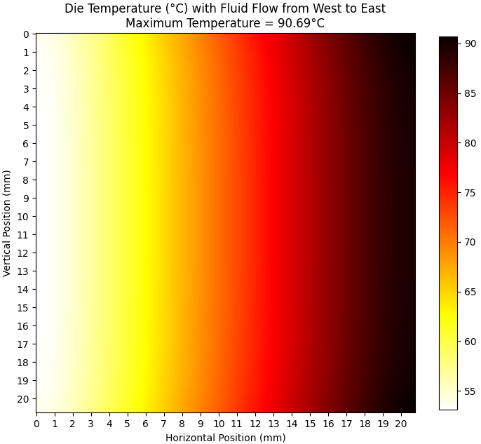
After deriving this circuit, HotSpot solves it using circuit analysis techniques like Kirchhoff's current law. Solving the circuit gives the temperature at every node (analogous to the voltage at every node in an electrical circuit), which corresponds to the temperature in every cell. Here is an example top-down heat map from HotSpot 6.0:

Lastly, let's take just a minute to discuss how HotSpot 6.0 models cooling (this will become more relevant when discussing my work in the next section). HotSpot 6.0 assumes that the sides of a chip are adiabatic, meaning that no heat can flow from the side of the chip to the ambient environment. HotSpot 6.0 does, however, model a heat spreader, thermal interface material (TIM), and a heat sink. These three parts of the chip's cooling solution are essentially modeled as thermal resistances that connect to the ambient, allowing heat to flow out of the chip to the ambient. To learn more about HotSpot, its thermal model, and especially the motivation behind its original creation, you can read the landmark paper that introduced HotSpot 1.0, "Temperature-Aware Microarchitecture".

My Work on HotSpot 7.0

The new functionality that I've added to HotSpot is in response to the increasing popularity of 3D Integrated Circuits (3D ICs). This new style of chip allows for decreased interconnect lengths, improved energy usage, and wider bandwidth, but it tends to have thermal challenges. When heat was produced over the surface of a 2D chip, it was fairly easy to remove with a heat sink. Now, since heat is being produced throughout a 3D volume, it's harder to extract out of one of the 3D IC's 2D surfaces. One of the popular solutions to this issue has been to use liquid cooling, but on a much smaller scale: microchannels can be made throughout a 3D IC to support cooling the chip from the inside. This approach is called microfluidic cooling.

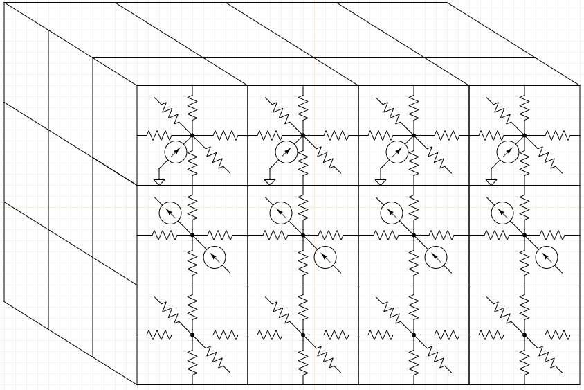
Like I mentioned before, HotSpot 6.0 can only model cooling via a heat sink. My work has been to add support for microfluidic cooling. To model a 3D IC, HotSpot 6.0 divides a 3D IC into an array of cells and then models each cell as a node in a thermal circuit. To model microfluidic cooling in HotSpot 7.0, I've added the distinction between solid cells and fluid cells. Solid cells in HotSpot 7.0 are treated the same as solid cells in HotSpot 6.0. For fluid cells, however, we need to model heat flow downstream due to the movement of the fluid through the microchannels. To model this, adjacent fluid cells are connected via heat sources (analogous to current sources in an electrical circuit). Here's a schematic in which the middle layer is composed of fluid cells:

There is an interesting challenge associated with this modeling methodology: if the microchannels are laid out in an interesting way (not just straight channels spanning the length of the chip), we don't know a priori how fast the fluid will be moving in a given channel. To solve this issue, we add another layer of abstraction: a pressure circuit in which all fluid cells are nodes. We model fluid flow using hydraulic resistances and by modeling the pump as a pressure source. Once this circuit has been constructed, it can again be solved using normal circuit analysis techniques. This gives us the pressure at each node in the pressure circuit, which corresponds to the pressure in each fluid cell. Once we know the pressure in every fluid cell, we can easily find the fluid flow rate between any pair of adjacent fluid cells. To summarize, we now have two abstraction layers: a pressure circuit and a thermal circuit. Once HotSpot 7.0 creates and solves a pressure circuit, it has information about fluid flow everywhere in the microchannels. It then uses these results to create and solve a thermal circuit.

Another major change that I've made in HotSpot is in the differential equations solver. HotSpot 6.0 used a solver based on the 4th-order Runge Kutta algorithm. This worked well for thermal circuits without microfluidic cooling, but it was prohibitively slow for thermal circuits that included microfluidic cooling. Furthermore, these circuits really can be massive: the connectivity matrix used to describe a recent simulation of mine was about 1.08 trillion by 1.08 trillion in size. To address this, I developed a new solver using the backward Euler method and the SuperLU sparse matrix library. The new solver was able to finish the aforementioned simulation in about 10 minutes.

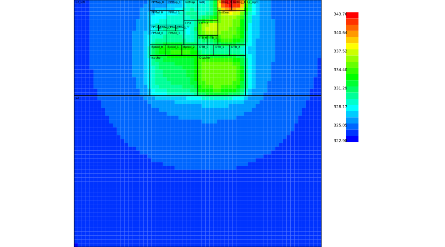
Finally, I've made a variety of smaller improvements. I simplified HotSpot's user interface in several ways. I also created a new visualization tool. Here is a heat map produced by HotSpot 7.0: